Sentiment Analysis with Pytorch — Part 3— CNN Model

7 min readApr 7, 2020

Introduction

This post is the third part of the series Sentiment Analysis with Pytorch. In the previous part we went over the simple Linear model. In this blog-post we will focus on modeling and training a bit more complicated architecture— CNN model with Pytorch.

If you wish to continue to the next parts in the serie:

Sentiment Analysis with Pytorch — Part 4 — LSTM\BiLSTM Model

Sentiment Analysis with Pytorch — Part 5— MLP Model

Building a CNN Model

The CNN (ConvNet) that we are going to build in this tutorial contains two convolutional layers, one with a kernel size equal to 3 and the other one with a kernel size equal to 8. Each convolutional layer is followed by a max pooling layer and a fully-connected layer with 256 units.

Our hyper-parameters:

lr = 1e-4
batch_size = 50
dropout_keep_prob = 0.5
embedding_size = 300
max_document_length = 100  # each sentence has until 100 words
dev_size = 0.8 # split percentage to train\validation data
max_size = 5000 # maximum vocabulary size
seed = 1
num_classes = 3
hidden_size = 128
pool_size = 2
n_filters = 128
filter_sizes = [3, 8]
num_epochs = 5

CNN Class

In the previous post I explained in detail about the general structure of the classes and the attribute inheritance from nn.Module. Here I focus on the CNN structure and each piece of code will be explained in detail .

Constructor

First, we will define all of the attributes of the CNN class in __init__ , and then we will define the forward pass by forward function:

import torch
import torch.nn as nn

class CNN(nn.Module):
    def __init__(self, vocab_size, embed_size, n_filters,                                                     filter_sizes, pool_size, hidden_size, num_classes,
                 dropout):
        super().__init__()        
        self.embedding = nn.Embedding(vocab_size, embed_size)
        self.convs = nn.ModuleList([nn.Conv1d(in_channels=1,
                                       out_channels=n_filters,
                                              kernel_size=(fs,    embed_size))
                                    for fs in filter_sizes])
        self.max_pool1 = nn.MaxPool1d(pool_size)
        self.relu = nn.ReLU()
        self.dropout = nn.Dropout(dropout)
        self.fc1 = nn.Linear(95*n_filters, hidden_size, bias=True)  
        self.fc2 = nn.Linear(hidden_size, num_classes, bias=True)  

    def forward(self, text, text_lengths):
        embedded = self.embedding(text)
        embedded = embedded.unsqueeze(1)       
        convolution = [conv(embedded) for conv in self.convs]   
        max1 = self.max_pool1(convolution[0].squeeze()) 
        max2 = self.max_pool1(convolution[1].squeeze())
        cat = torch.cat((max1, max2), dim=2)      
        x = cat.view(cat.shape[0], -1) 
        x = self.fc1(self.relu(x))
        x = self.dropout(x)
        x = self.fc2(x)  
        return x

Embedding Layer

Embedding layer creates a look up table where each row represents a word in a numerical format and converts the integer sequence into a dense vector representation.

There are two parameters that we need to transfer the embedding layer in the initialization level :

vocab_size: Number of unique words in the dictionary.
embed_size: Number of dimensions for representing a single word.

In the forward pass, the embedding layer receives the text dimensions in a shape of [batch size, sentence length] (In the first blog-post we set the variable batch_first=TRUE). After the text passes in the embedding layer it changes to the shape [batch size, sentence length, embedding dim]. For the next layer we will need to add another dimension because Conv1 gets 4-dimensions. We will use unsqueeze(1) function that will add 1 to the 1st dimension (which is not really matter to our calculations but it fits the tensor the next layer).

Squeeze

squeeze function reduces 1-length dimensions from the tensor (it is possible to mark which dimension exactly using the dim argument). For example, for the following input form: AX1XBXCX1XD, the function squeeze(input) will return the output AXBXCXD , and when dim is indicated squeeze(input, dim = 1) it will return AXBXCX1XD .

Unsqueeze

unsqueeze function adds a 1-length dimension to the tensor instead of dim dimension. dim argument ranges (-input.dim() - 1, input.dim() + 1) , if dim gets a negative value the dimension will be (dim+input.dim()+1).

Convolutional Layer

After unsqueeze, we will get the input for the Conv1d in the shape [batch size, 1, sentence length, embedding dim]. We will use nn.ModuleList to build a list of Conv1d (when a filter slides along a single dimension) that can get a list of different filter sizes and it will create convolutional layers for each of the filters.

The function Conv1d has few arguments: in_channels , out_channels , kernel_size.

in_channels variable will get as an input the amount of channels the operation of the convolution is going to be executed on. For example, a channel can be used as the RGB color when we use images and we want to know whether the convolution applies to each color individually or all together. When we work with text or audio for example we will have just one channel.

out_channels is the number of output channels after the convolution operation was performed on the input matrix. Usually will be composed of the amount of filters that we want to use.

kernel_size will be initialized to the filter size that we will set on the Y-axis and the embedding size for the X-axis. We are working with words that each row in the matrix represents a different word, so the kernel width will be in the same dimension like the embedding dimension (to cover all the word) and the kernel size will be the length that will set between how many words in the sentence we want to find correlations. If kernel_size=2 so we will be working with bi-grams and will try to find correlations between each two words. For each language it works different so it’s better to check different sizes and to merge them later with the pooling operation.

The output dimension that we will get after the convolution, will be [batch size, number of filters ,n_out, 1].

n_in = sentence length, k = kernel size, p = padding size, s = stride size

Pooling Layer

After each convolutional layer, we apply nn.MaxPool1d with a pooling window of 2 to reduce the dimensionality. nn.MaxPool1d receives as an input a 3D tensor with a shape [batch size, number of filters ,n_out] , thus we will use squeeze to reduce the 1-sized dimensions before entering the max pooling function.

After nn.MaxPool1d the output will be of the shape [batch_size, number_of_filters ,n_out/pooling_window_size].

When we work with words, we need to use only 1-dimension, so after the Conv1d operation we will get a vector, so compared to images here we don’t need to flatten anything and we will compute thenn.MaxPool1d on each vector to get one value that will be merged later with torch.cat function.

Cat Function

torch.cat((t1, t2), dim=0) concatenates the tensors by dim dimension. In our case we want to concatenate the tensors from the two different kernels that we used by the second dimension. The output shape will be of the form [batch_size, number_of_filters ,n_out1/pooling_window_size + n_out2/pooling_window_size]

View Function

Next, we will flatten the tensor using view function that reshapes the tensor to a different size. For example, let’s create a random tensor of size 2X3:

x = torch.randn(2, 3)tensor([[-0.3686, 1.4924, -1.0179],[ 0.4780, 2.1494, -0.0446]])

And resize it to 1X6:

y = x.view(6)
tensor([-0.3686,  1.4924, -1.0179,  0.4780,  2.1494, -0.0446])

dim argument that is equal to -1 will complete the missing dimension automatically. For example, for tensor x , -1 will be equal to 3:

z = x.view(-1, 2)tensor([[-0.3686, 1.4924],[-1.0179, 0.4780],[ 2.1494, -0.0446]])

We will use this function to flatten the tensor for each sample in the batch so the output shape will be of the following form:

[batch_size, (number_of_filters) X (n_out1/pooling_window_size + n_out2/pooling_window_size)]

Activation Function

We used the ReLU function in this model that does not change the original dimensions.

Fully-Connected Layer

nn.Linear is also called a fully-connected layer or a dense layer, in which all the neurons connect to all the neurons in the next layer. The dimension of the output shape after the first fully-connected layer will be of the form [batch_size, hidden_size] , and after the second fully-connected layer will be as following[batch_size, num_of_classes] .

Dropout Layer

The dropout layer randomly dropping out units in the network. Since we chose a rate of 0.5, 50% of the neurons will receive a zero weight. This operation controls the regularization process and helps in preventing overfitting. nn.Dropout will not change the dimensions of the original input.

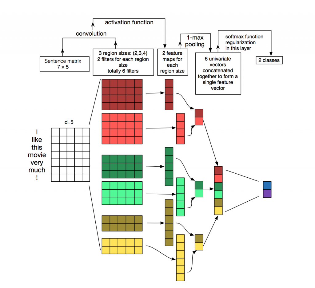
Here you can see an example of what we explained above in the diagram below and read more on CNN with NLP in this article.

Training, Evaluation and Test

The training, evaluation and test are exactly the same in all of the models. In the previous post we explained in detail all of those steps so you can read more about it here.

Main Function

import torch
import os

if __name__ == "__main__":
    device = torch.device('cuda' if torch.cuda.is_available() else 'cpu')
    path = 'C:/Users/Gal/PycharmProjects/Sentiment_Analyzer'
    path_data = os.path.join(path, "data")

    model_type = "CNN"
    data_type = "token"  # or: "morph"

    char_based = True
    if char_based:
        tokenizer = lambda s: list(s)  # char-based
    else:
        tokenizer = lambda s: s.split()  # word-based

    lr = 1e-4
    batch_size = 50
    dropout_keep_prob = 0.5
    embedding_size = 300
    max_document_length = 100  # each sentence has until 100 words
    dev_size = 0.8  # split percentage to train\validation data
    max_size = 5000  # maximum vocabulary size
    seed = 1
    num_classes = 3
    hidden_size = 128
    pool_size = 2
    n_filters = 128
    filter_sizes = [3, 8]
    num_epochs = 5    Text.build_vocab(train_data, max_size=max_size)
    Label.build_vocab(train_data)
    vocab_size = len(Text.vocab)

    train_iterator, valid_iterator, test_iterator = create_iterator(train_data, valid_data, test_data, batch_size,
                                                                    device)

    loss_func = nn.CrossEntropyLoss()
    cnn_model = CNN(vocab_size, embedding_size, n_filters, filter_sizes, pool_size, hidden_size, num_classes,
                    dropout_keep_prob)

    optimizer = torch.optim.Adam(cnn_model.parameters(), lr=lr)
    run_train(num_epochs, cnn_model, train_iterator, valid_iterator, optimizer, loss_func, model_type)
    cnn_model.load_state_dict(torch.load(os.path.join(path, "saved_weights_CNN.pt")))
    test_loss, test_acc = evaluate(cnn_model, test_iterator, loss_func)
    print(f'Test Loss: {test_loss:.3f} | Test Acc: {test_acc * 100:.2f}%')

End Notes

In this section we built CNN model with Pytorch. In the next parts we will learn how to build LSTM and BiLSTM models in Pytorch for Sentiment Analysis task. If you wish to continue to the next part, here you can find the link for the next section in the serie: Sentiment Analysis with Pytorch — Part 4— LSTM\BiLSTM Model.

You can find the full code for this tutorial on Github.